Pivot Chart
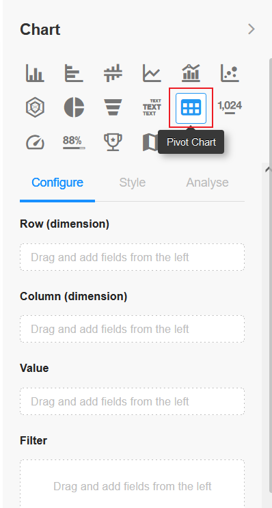
Features: A pivot chart is an interactive table for quickly summarizing data with cross-tabulations. It helps users to analyze and organize data.
The following is an example of how to create a pivot chart.
Example: In the worksheet Sales, create a chart to analyze and display the sales of this month
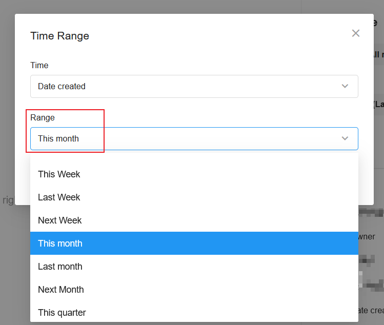
Data range: Sales records in this month
Filtering field: Date created
Time range: This month
Numeric: Region, Product, Date, Amount
1. Create a new chart
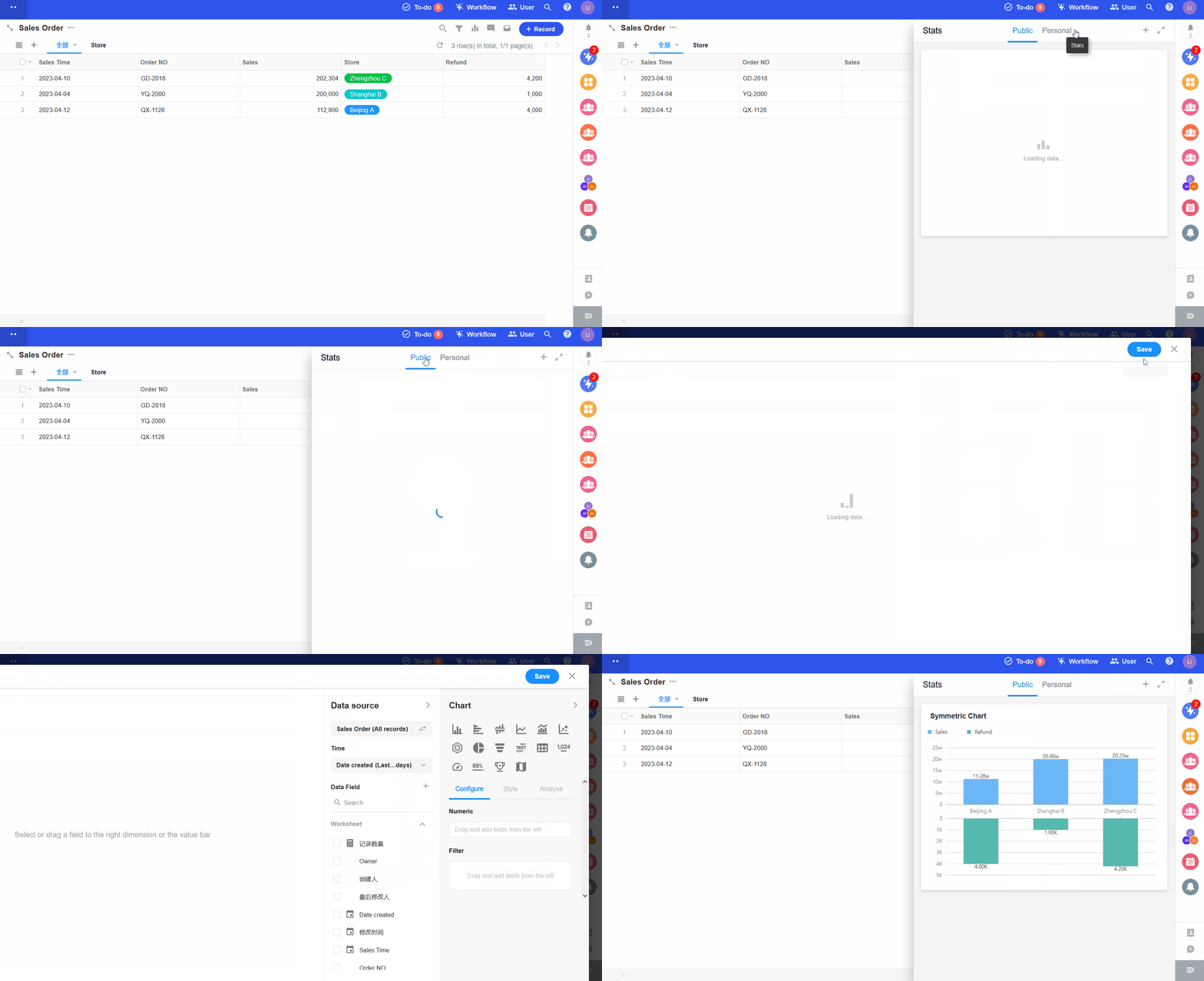
2. Set the data source
3. Select the [Pivot Chart]
4. Set the dimension
Row: region, product
Column: date (day)
Numeric: total sales amount
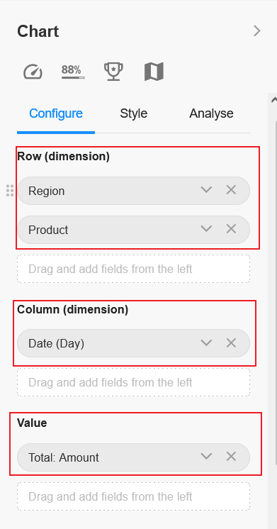
When setting the dimension, you can set the display field of the associated worksheet if you select the field in the associated worksheet.
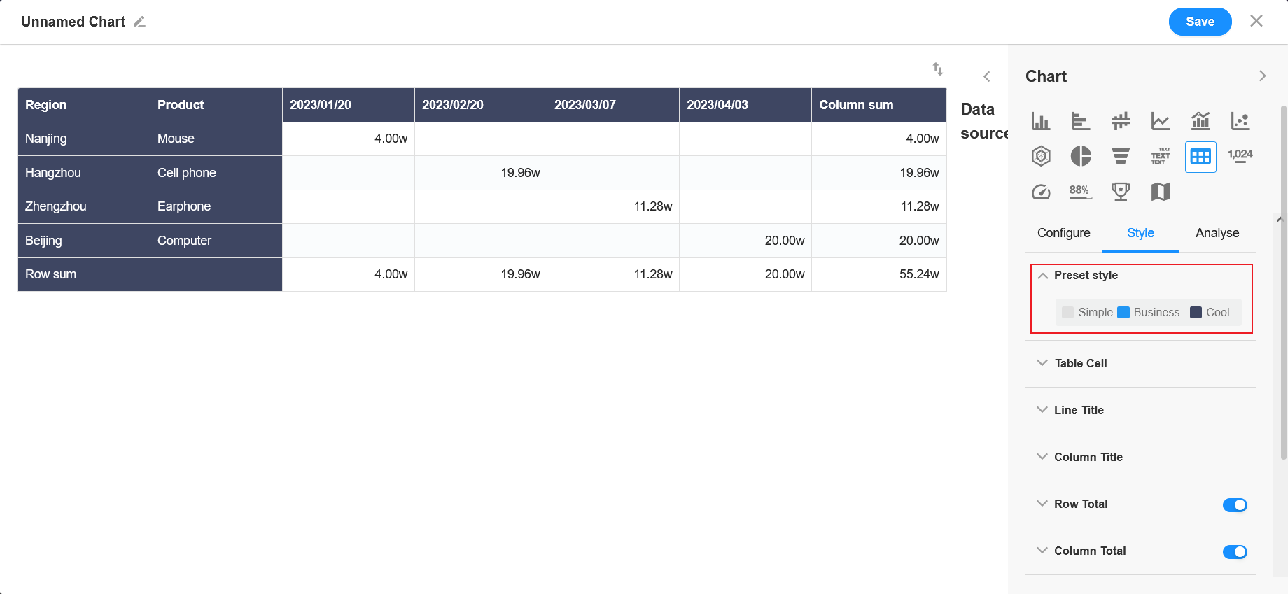
5. Preset style
Set the color of the row or column header.
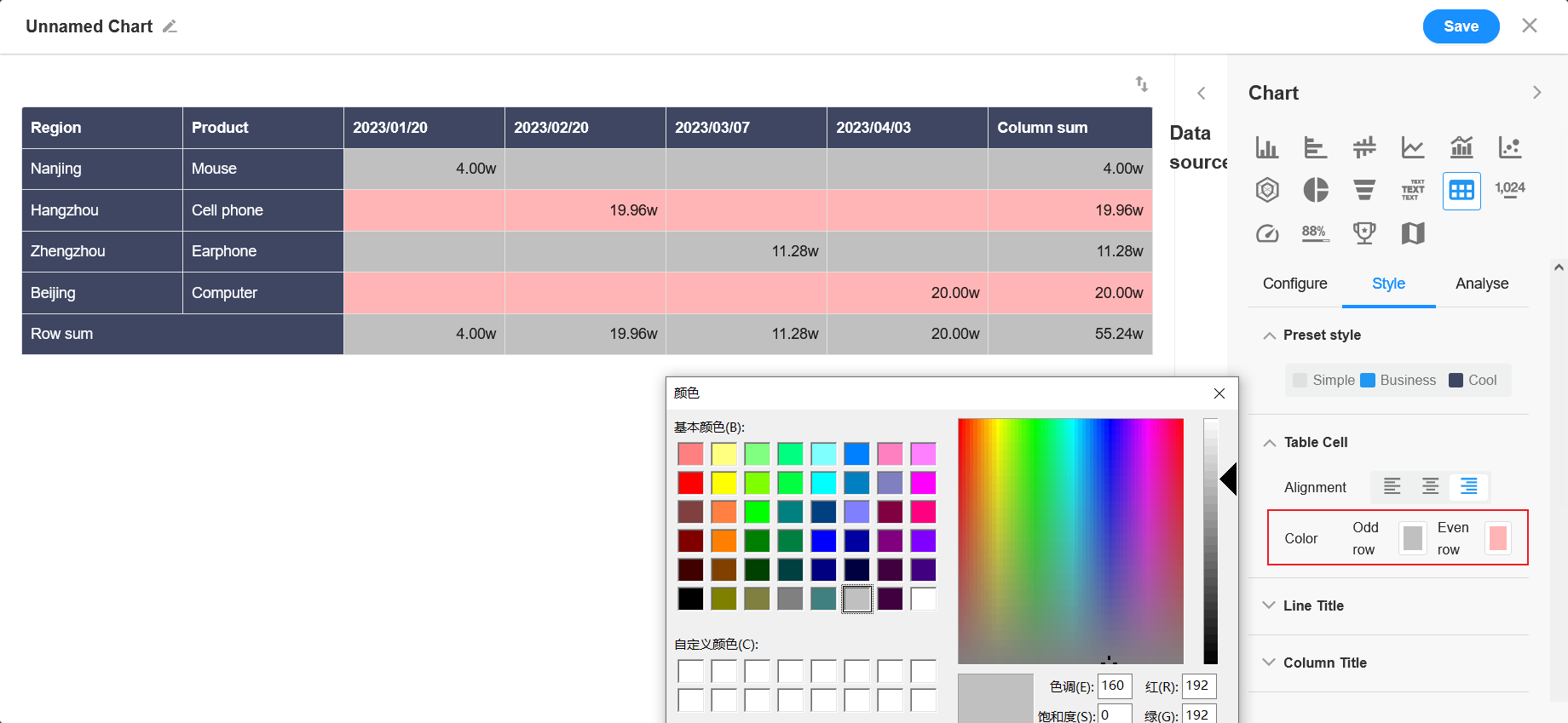
6. Cell
Here set the color of the cell and how to display it.
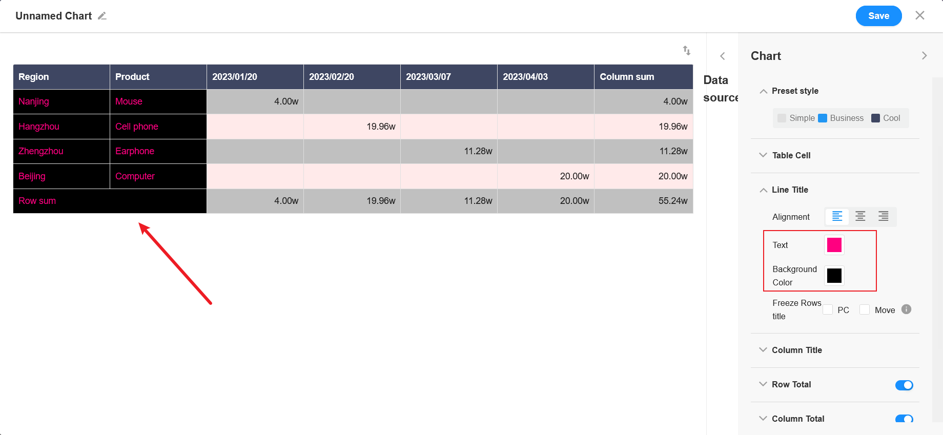
7. Row/Column title
In the preset style, you can also set the color of the table header, alignment and background color.
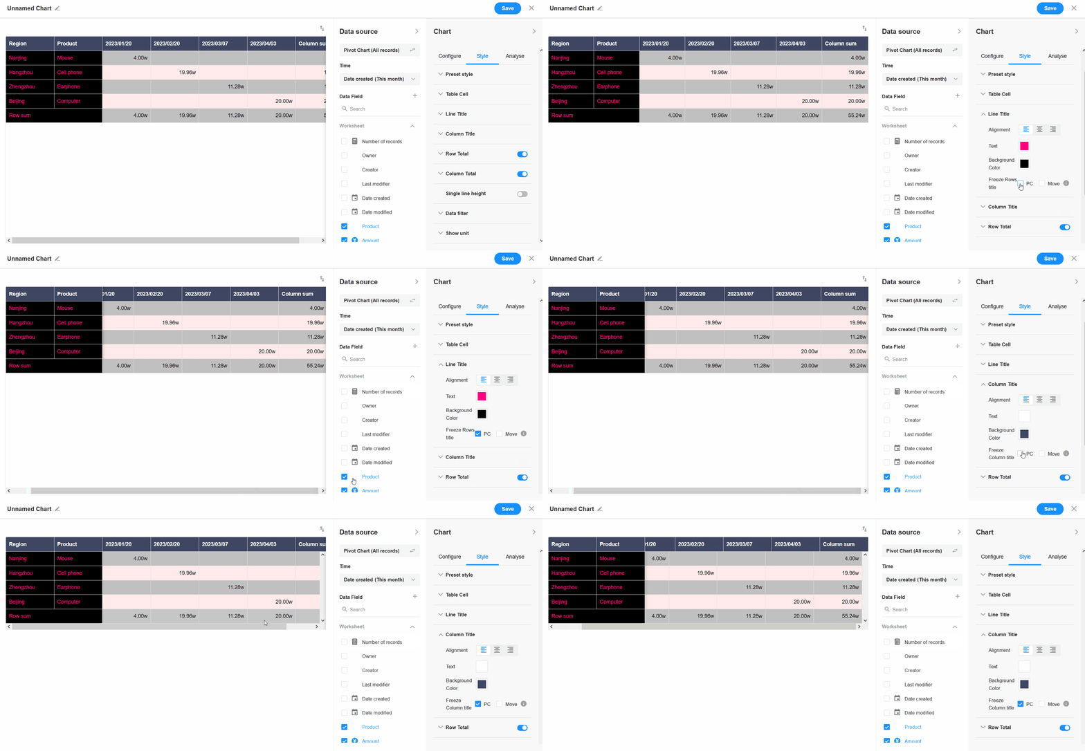
Whether to freeze the row/column headers on pc or mobile.
8. Display settings
Here set whether to enable row totals or column totals and how to display them.
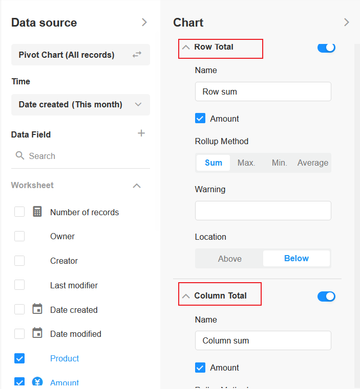
For row totals or column totals, you can set the rollup method depending on the selected field, which may be different for each field.
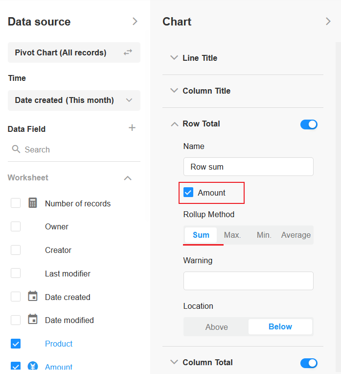
Name: click to modify
Hint: you can set to add some hints in front of the field
Location: you can set the placement of the summary column
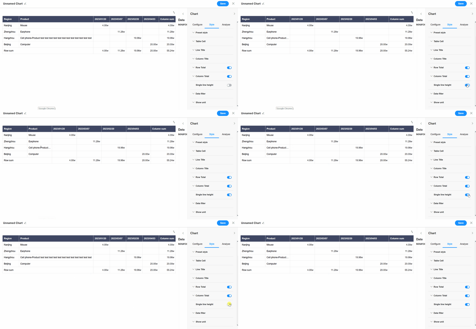
9. Single line height
In the pivot chart, it defaults to adaptive height to display the full content. If enabled [single row height], it will fix the line height to show only one line of content, and the content beyond will be displayed as an ellipsis.
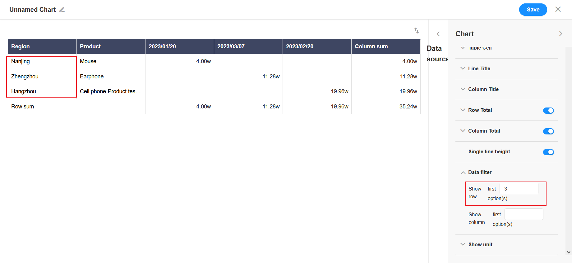
10. Data filtering
You can set to show only the first X items of the row or column.
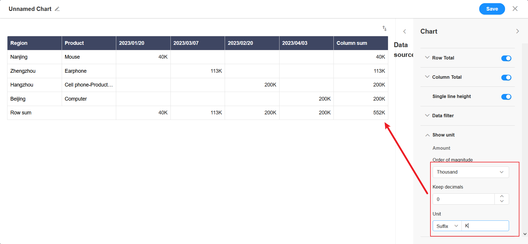
11. Show unit
For numeric fields, you can set the unit and the number of decimal places.
12. Save
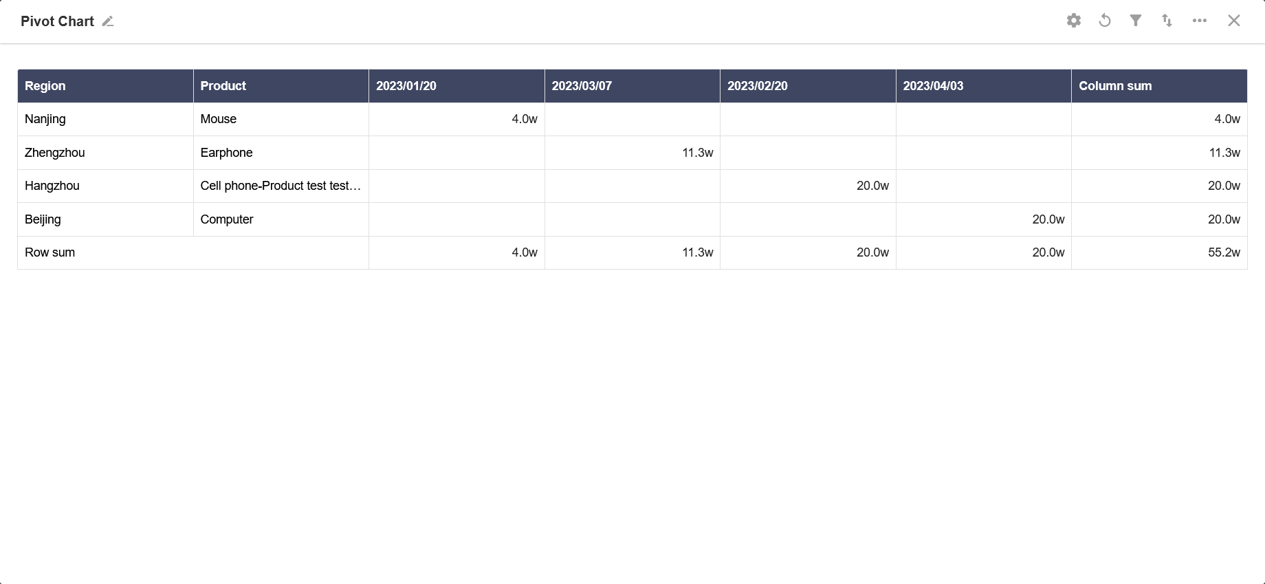
Effect:
Have questions about this article? Send us feedback